
Time series data is a record of sequential data measured at a regular time-intervals over a period of time. These data are used to extract any meaningful statistics and other characteristics. Time series are mostly non-stationary data, used to build a model that predict future values based on previously observed values. There are plenty of methods for forecasting retail sales, now we are going to see some of these methods one by one.
The Dataset
To demonstrate forecast methods, we are going to use monthly sales data of shampoo for 3 year period as data set.
| Name | description |
|---|---|
| Dataset title | Sales of shampoo over a three year period |
| Dataset metrics | 36 fact values in 1-time series. |
| Source | Datamarket.com |
Visualizing shampoo sales time series data
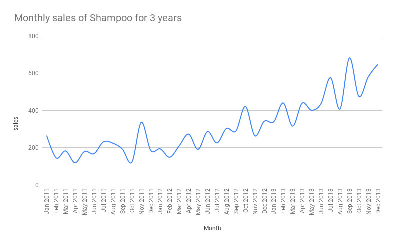
Some of the patterns appearing in the plotted data:
Every year from September to December there is a bump in the sales shows the seasonality pattern, overall sales trend is increased when compared to the year 2011 and 2013 sales. There is an upward trend in overall sales even though many low months in between.
Sales forecasting methods
Let us do practical analysis by applying most commonly used time series forecasting methods. Depending on sales data, some forecasting methods will perform better than others for a given historical data set. A forecasting method that is appropriate for one product may not be appropriate for another product. Depending on the product life cycle position some forecasting methods may provide good results and it may not continue throughout the life cycle.
Performance Evaluation
To evaluate these forecasting methods, we need to calculate Mean Absolute Deviation (MAD) and Percent of Accuracy (POA). Both of these performance evaluation methods require historical sales data for a user-specified period of time. This period of time is called a holdout period or periods best fit (PBF). The data in this period is used as the basis for recommending which of the forecasting methods to use in making the next forecast projection.
Calculating Percent of Accuracy (POA)
For period = n
                                    ( Forecast value of period 1 ) + …..  + (Forecast value of period n )
     POA           =        ------------------------------------------------------------------
                                    ( Actual value of period 1 ) + …… + (Actual value of period n )
Calculating Mean Absolute Deviation (MAD)
For period = n
            ( |Forecast value of period 1 - Actual value of period 1| ) + ….. + ( |Forecast value of period n - Actual value of period n| )
 MAD =  -------------------------------------------------------------------------------------------------------------------
                                                                                    n
1. User-specific percent over previous period - Forecast method
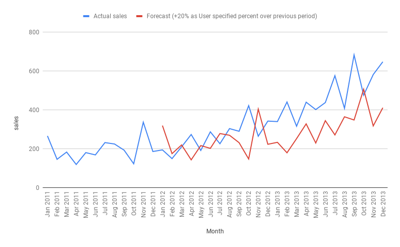
In this forecast, method user can specify percentage to multiplies sales data from the previous year. In this example, we used 1.20 for 20% increase as forecast.
Required data :
- At least 1 year of previous year sales data.
- The user-specific number to calculate forecast.
- User-specified number of time periods for evaluating forecast performance
Performance Evaluation
- Calculated for 3 months period
- Percent of Accuracy Calculation (POA) = 98.91
- Mean Absolute Deviation (MAD) = 127.15
- Periods best fit (PBF) is from May 2012 to July 2012
2. Calculated percent over previous period - Forecast method
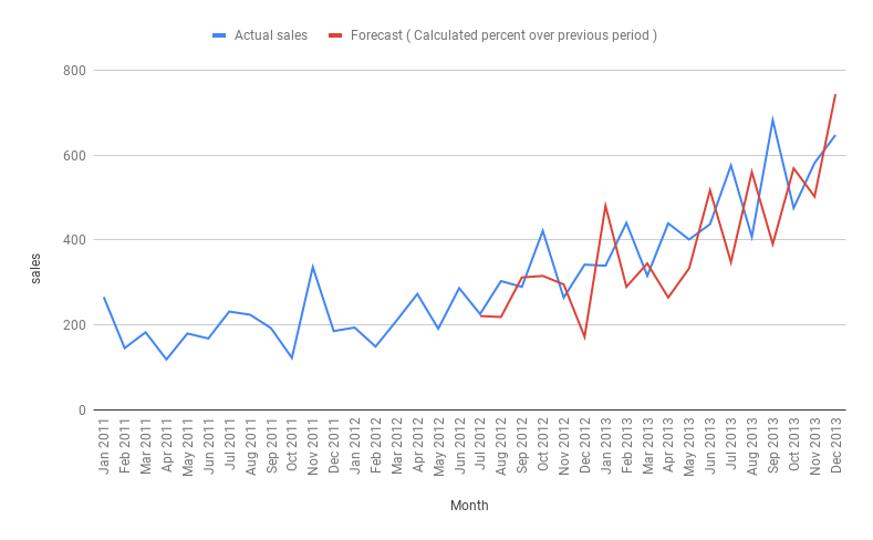 This forecasting method will calculate the percentage from the last 2 years sales data and then apply the same to calculate the forecast.
Required data :
- At least 2 years of previous years sales data.
- User-specified number of time periods to calculate the percentage and evaluating forecast performance
Calculation :
- Number of time periods = 6
- Forecast percentage = Sum from Jan 2012 to June 2012 / Sum of Jan 2011 to June 2011
- Forecast value July 2012 = (Previous sales value) x (Forecast percentage)
Performance Evaluation
- Calculated for 3 months period
- Percent of Accuracy Calculation (POA) = 91.83
- Mean Absolute Deviation (MAD) = 96.58
- Periods best fit (PBF) is Jul 2012 to Sep 2012
3. Previous period as current period - Forecast method
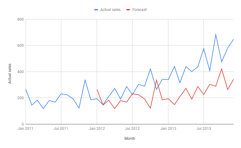 Using last year sales value as forecast value.
Required data :
- At least 1 years of previous years sales data.
- User-specified number of time periods to evaluating forecast performance
Performance Evaluation
- Calculated for 3 months period
- Percent of Accuracy Calculation (POA) = 107.42
- Mean Absolute Deviation (MAD) = 84.30
- Periods best fit (PBF) is Jan 2012 to Mar 2012
4. Moving Average - Forecast method
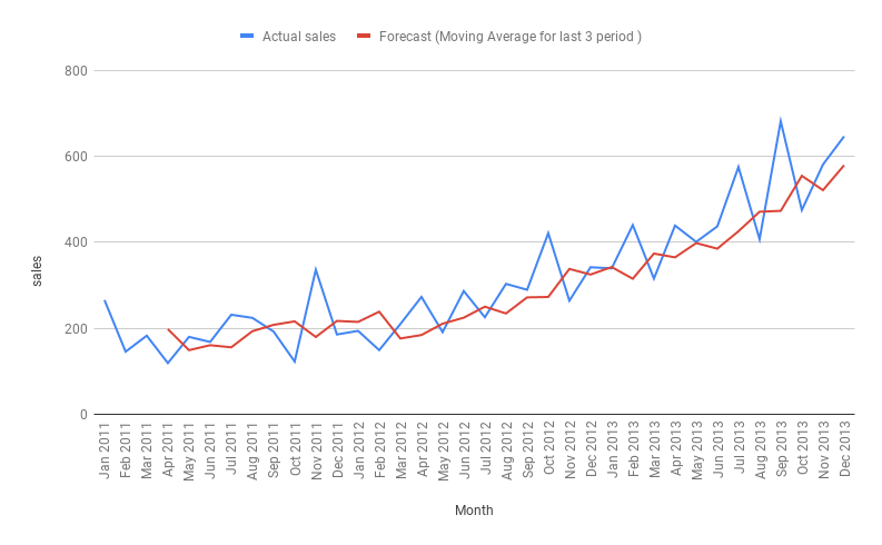
Moving Average forecast method will average user-specified number of months sales data and forecast the next month demand.
Required data :
- User-specified number of time periods to calculate the percentage and evaluating forecast performance
- At least double a specified number of months sales data. (i.e) If the specified period is 3 then we need 6 months sales data
Calculation :
Number of time periods = 3
Forecast value Apr 2011 =  Sum of Jan 2011 to Mar 2011  /  3
Forecast value of current month =  Average of last 3 months sales value
Performance Evaluation
- Calculated for 3 months period
- Percent of Accuracy Calculation (POA) = 97.45
- Mean Absolute Deviation (MAD) = 89.82
- Periods best fit (PBF) is May 2012 to Jul 2012
5. Linear Approximation - Forecast method
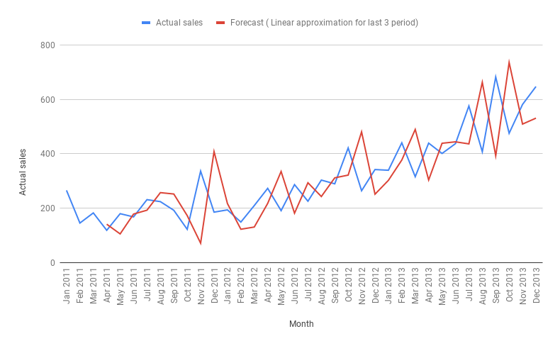
Linear Approximation calculates a trend based upon two sales history data points. Those two points define a straight trend line that is projected into the future.
Required data :
- The number of periods to include in the regression
- At least double the specified number of months sales data. (i.e) If the specified period is 3 then we need 6 months sales data
Calculation :
Number of time periods = 3
Forecast value Apr 2011 = ( [sales of Mar 2011 - sales of Jan 2011] /  2 ) + sales of Mar 2011
To forecast next one year period i.e for next 12 month:
Forecast value Jan 2014 =  ([sales of Oct 2013 - sales of Dec 2013] / 2) x 1  + sales of Dec 2013
Forecast value Feb 2014 =  ([sales of Oct 2013 - sales of Dec 2013] / 2) x 2  + sales of Dec 2013
       ,,
       ,,
Forecast value 12th month =  ([sales of Oct 2013 - sales of Dec 2013] / 2) x 12  + sales of Dec 2013
Performance Evaluation
- Calculated for 3 months period
- Percent of Accuracy Calculation (POA) = 93.28
- Mean Absolute Deviation (MAD) = 90.40
- Periods best fit (PBF) is May 2013 to Jul 2013
6. Least Square Regression - Forecast method
One of the most popular methods to determine linear trend using historical sales data is Linear Regression or Least Squares Regression (LSR). The method calculates the values of a and b to be used in the formula: Y = a + b X
Required data :
- The number of periods to include in the regression
- At least double the specified number of months sales data. (i.e) If the specified period is 3 then we need 6 months past sales data
Calculation :
Number of time periods (n) = 3
This table is to calculate Linear Regression Coefficients, given n = 3:
| Month Year | Period (i) | Sales(j) | ij | i^2 |
|---|---|---|---|---|
| Oct 2013 | 1 | 475.3 | 475.3 | 1 |
| Nov 2013 | 2 | 581.3 | 1162.6 | 4 |
| Dec 2013 | 3 | 646.9 | 1940.7 | 9 |
| Σi= 6 | Σj =1703.5 | Σij = 3578.6 | 14 |
b = (nΣij – ΣiΣj) / [nΣi^2 – (Σi)^2]
b = [(3x3578.6) – (6×1703.5)] / [3 (14) – (6)^2]
b = (10735.8 – 10221) / (42 – 36)
b= 85.8

a = (Σj / n) – b (Σi / n)
a = (1703.5 / 3) – [(85.8)(6/3)]
a = 396.2

Y = a + b X    i.e X is period number to be forecast with the sequence to existing period

To forecast next one year period i.e for next 12 month:
Forecast value Jan 2014  (Y) =  396.2 + (85.8 x 4)  =
        Here X = 5   i.e period number for Oct 2013 is 1, then the period number for Jan 2014 is 4

Forecast value Feb 2014 (Y) =  596.2 + (85.8  x 6) =
        Here X = 5   i.e period number for Oct 2013 is 1, then period number for Feb 2014 is 5
       ,,
       ,,

Forecast value nth period ( Y) =   596.2 + 85.8 x n
Performance Evaluation
- Calculated for 3 months period
- Percent of Accuracy Calculation (POA) = 97.37
- Mean Absolute Deviation (MAD) = 43.81
- Periods best fit (PBF) is Jun 2011 to Aug 2011
Conclusion
The main objective here is to do some effective forecasting sales data especially when more than one dimensions exist, we need to set up multiple forecasting for each dimension level and also for different product life cycle stages. Some more forecasting methods will be discussed in coming articles.