Time series forecasting with ARIMA using two different data sets

Introduction

Time series analysis ARIMA Forecasting using python stats models - Seasonal Autoregressive Integrated Moving-Average with eXogenous regressors (SARIMAX) for two different data sets

1. Shampoo sales data 3 years of monthly data (source)

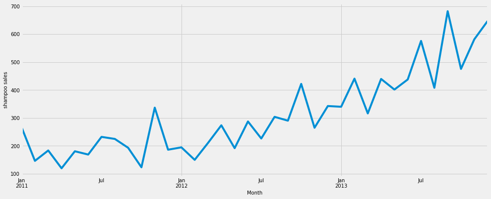
Observations:

1. 3 years of historical data
2. Very less sign of seasonal factor

3. Year on year growing trend is high

4. Milk production data 14 years of monthly data (source)

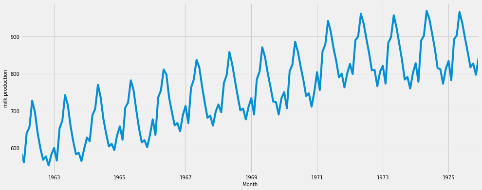
Observations:

1. 3 years of historical data
2. The very high seasonal factor
3. Year on year growing trend is slow and steady ( stable )

Visualize season, trend & residual

Using seasonal decompose function in stats models time series analysis

decomposition = sm.tsa.seasonal_decompose(y, model='additive')

This function decompose any time series into three distinct components trend, seasonality, and noise

Decompose of Shampoo sales

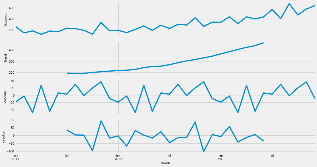
Observations:

1. The trend starts at below 200 reaches above 500
2. Identical seasonal index in each year
3. High noise level ( -100 to +100)

Decompose of Milk production

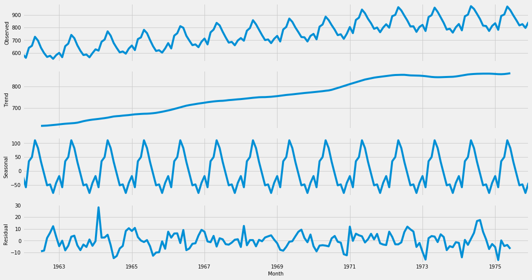
Observations:

1. The trend starts at below 700 reaches above 800
2. Exactly identical seasonal index in each year
3. Noise level very low ( -10 to +30) by comparing shampoo sales data

Models and Estimation

The following are the main estimation classes, which can be accessed through stats models.tsa.statespace.api and their result classes. Seasonal Autoregressive Integrated Moving-Average with eXogenous regressors (SARIMAX) is a widely used model for better prediction.

mod = sm.tsa.statespace.SARIMAX(y,
                                order= param_1,
                                seasonal_order= param_2 ,
                                enforce_stationarity=False,
                                enforce_invertibility=False)

Finding the optimal parameters

Before going into the model we need to find the optimal set of parameters We need to find the optimal set of parameters that will yield the best prediction model. Order = param_1 Seasonal_order = param_2 By runing the model with all (0,1) combination and find the lowest AIC value for which param

optimal parameters of Shampoo sales data order=(1, 0, 1), seasonal_order=(1, 1, 0, 12),

optimal parameters of milk production data order=(0, 1, 1), seasonal_order=(0, 1, 1, 12),

Fitting the model

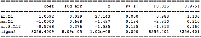
Using the optimal params for respective data set, now fit with SARIMAX model we get the following results.

For shampoo sales data

For Milk production data

Model diagnostics

Before running the prediction model we need to do the model diagnostics to find any unusual behavior with the given data using the following python function.

Mod.fit.plot_diagnostics

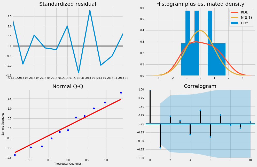
Diagnostics Shampoo sales data

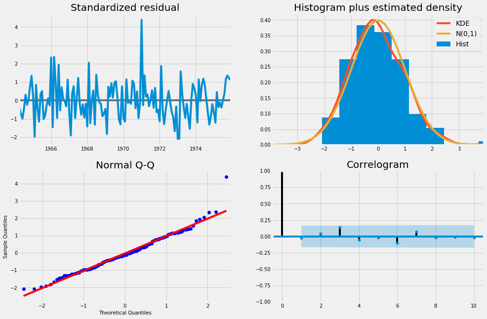
Diagnostics Milk production data

Forecasting for one year to validate

Validation of the forecast helps to understand the accuracy. compare the predicted value with an observed value of the time series. Last one year data with actual (blue line) and calculated forecast (red line). Grey area shows the lower limit & upper limit of the prediction

pred = results.get_prediction(start=pd.to_datetime('yyyy-mm-dd'), dynamic=False)

Shampoo sales

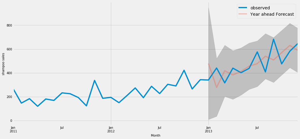
Observations:

1. Prediction value rarely matched with actual data
2. The grey background in the graph shows the upper and lower limit of the prediction range is very high (-350 to +450 )

Milk production

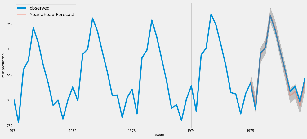
Observations:

1. Prediction value mostly matched with the actual data.
2. The grey background in the graph shows the upper and lower limit of the prediction range is very low ( - 50 to +50 ) that shows the good prediction model.

Mean Squared Error

Performance Evaluation for this prediction model is MSE calculated using the following function

mse = ((y_forecasted - y_truth) ** 2).mean()

Smaller the MSE will give the best accuracy of the predicted value. In Shampoo sales data The Mean Squared Error of our forecasts is (MSE): 10975.99 The Root Mean Squared Error of our forecasts is (RMSE): 104.77 (Square root of MSE is RMSE)

Milk production data The Mean Squared Error of our forecasts is (MSE): 36.65 The Root Mean Squared Error of our forecasts is (RMSE): 6.05

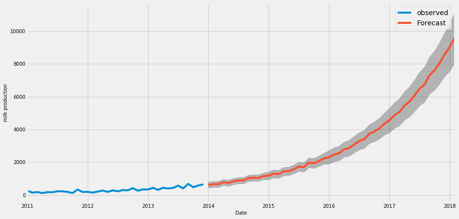
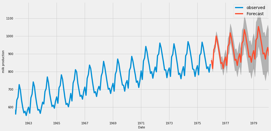
Future Forecast:

To predict the future for 50 steps using the following get_forecast() function

predict _50_steps_ahead = results.get_forecast(steps=50)

Shampoo sales data

Milk production data

Conclusion

From the above analysis, we can say more historical data in time series will help us to predict more accurately. Also, we can see the seasonal factor exactly comes into the predicted value in the milk production data. However, in shampoo sales data the seasonal factor is not visible as like others.

References:

https://www.statsmodels.org/stable/statespace.html#seasonal-autoregressive-integrated-moving-average-with-exogenous-regressors-sarimax

https://www.digitalocean.com/community/tutorials/a-guide-to-time-series-forecasting-with-arima-in-python-3