
This article will illustrate more forecast methods other than covered in part 1. however, we are going to use the same dataset. Let’s get into the models one by one. For each method, the demonstration is organized in the following way, Formula, calculation, illustrated graph and Performance Evaluation.
Second Degree Approximation - forecast method
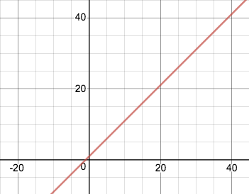
In Linear Regression determines values for a and b in the forecast formula. Desmos online tool helped me to visualize this formula Y = a + b X. this formula helps us to fit a straight line to the sales history data.
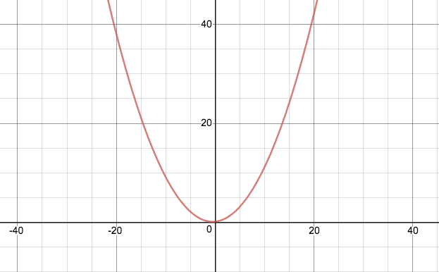
 However, in Second Degree Approximation using this formula Y = a + b X + c X 2 by visualizing this
Required data :
- At least 3 quarters periods of sales data (i.e) need 9 months sales data
- Specific Number of months to evaluate. ( example 3 months)
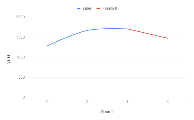 Convert monthly sales history to quarterly data to fit a curve. Now we get above formula fits into each point as follows. To forecast using this method we need to determines values for a, b, and c.
Calculation :
  Y = a + bX + cX2
  Apply X =1 for Q1 , X = 2 for Q2 and X=3 for Q3
  Q1 = a + b + c          ………..(1)
  Q2 = a + 2b + 4c      ………..(2)
  Q3 = a + 3b + 9c     ………...(3)
  Solve the three equations simultaneously to find b, a, and c:
   a = Q3 – 3(Q2 – Q1)                      =    649.1 - 3 (468.1 - 595)                =   1029.8
   b = (Q2 – Q1) –3c                        =    (468.1 - 595) - 3c                     =    -860.25
   c = [(Q3 – Q2) + (Q1 – Q2)] / 2          =    [(649.1 - 468.1) + (595 - 468.1)] / 2  =  244.45
 This is a calculation of second degree approximation forecast:
   Y = a + bX + cX2 = 1029.8   + (-860.25)X +(244.45) X2
   To forecast Q4 , replace value of X = 4, Q4 = 1470. The forecast per period  Q4 / 3  = 490.00
   To forecast Q5 , replace value of X = 5, Q5 = 926.2. The forecast per period  Q5 / 3 = 308.73
   To forecast Q6 , replace value of X = 6, Q5 = 72.1 The forecast per period  Q6 / 3   = 24.03
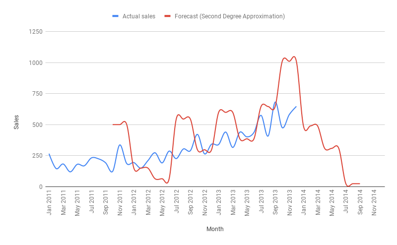
Performance Evaluation
- Calculated for 3 months period
- Percent of Accuracy Calculation (POA) = 100.25
- Mean Absolute Deviation (MAD) = 90.58
- Periods best fit (PBF) is May 2013 to Jul 2013
We can use this method, while a product is in the transition stages of the product life cycle. like, a new product moves from a launch period to growth stages, acceleration of sales trend may increase. However, this method is useful only in the short term. Because of the next level forecast can quickly approach very high or down to zero.
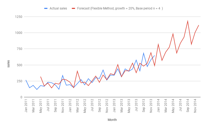
Flexible Method - forecast method
The Flexible Method is similar Percent Over Last Year method. But the user can have to decide the percentage and how many months prior (n). By multiple sales data from a previous time period by a user specified factor that result in the future. This method gives the capability to specify a time period other than the same period last year.
Required data:
- Forecast percentage i.e. Multiplication factor. For example, 1.20 means increase the previous sales history data by 20%.
- Base period (n). For example, n = 4 will cause the Jan forecast to be based upon sales data in September of last year.
- At least 8 months historical sales data. Number of periods back to the base period, and the number of time periods required for evaluating the forecast performance
(PBF).
Calculation :
In this example user specified base period n = 4 and growth (or) decline percentage = 1.20
(Note: 1.20 means 20% growth, if the value is 0.80 then 20% decline)
Sales forecast of Jan 2014 =  sales value of  [ Last month (dec 2013) - Base period(4) ] x 1.20
                                            =  sales value of Sep 2013 x 1.20
   ,,
   ,,
Sales forecast of May 2014 =  Forecasted sales value of Jan 2014 x 1.20
Performance Evaluation
- Calculated for 3 months period
- Percent of Accuracy Calculation (POA) = 103.90
- Mean Absolute Deviation (MAD) = 31.45
- Periods best fit (PBF) is Nov 2012 to Jan 2013
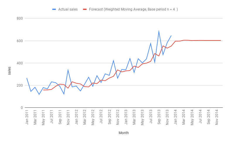
Weighted Moving Average - forecast method
This method is similar to the Moving Average. However, with the Weighted Moving Average, the user can assign unequal weights to the historical data. The method calculates a weighted average of recent sales history to arrive at a projection for the short term. More recent data is usually assigned a greater weight than older data, so this makes WMA more responsive to shifts in the level of sales.
Required data:
- Base period (n). the number of periods of sales history to use in the forecast calculation. For example, specify n = 4 here moving average will be calculated from the past 4 periods.
- The weight assigned to each of the historical data periods. assign weights of 0.4, 0.3, 0.2, and 0.1 with the most recent data receiving the greatest weight. (other
options 0.50, 0.25, 0.15, and 0.10 | .45, .25, 0.20, 0.10 )
Calculation :
In this example user specified-base (n) = 4 and weights must total 1.00. When Base period n = 4, split the weight into 4 values. I.e. assign weights of 0.4, 0.3, 0.2, and 0.1 with the most recent data receiving the greatest weight. To forecast the sales of Jan 2014 with base period n = 4, start from Last Sep [ Last month (Dec 2013) - Base period(4) ] to Dec apply the greatest weight to most recent data like below
        (sales value Sep x 0.1 ) + ( s.v. Oct x 0.2 ) + ( s.v. Nov x 0.3 ) + (s.v. Dec x 0.4)
   =   -----------------------------------------------------------------------------------------------------------------
                                        ( 0.4 + 0.3 + 0.2 + 0.1 )
      ,,
      ,,
 To forecast the sales of May 2014

           (forecast value Jan x 0.1 ) + ( f.v. Feb x 0.2 ) + ( f.v. Mar x 0.3 ) + (f.v. Apr x 0.4)
   =   -----------------------------------------------------------------------------------------------------------------
                                       ( 0.4 + 0.3 + 0.2 + 0.1 )
Performance Evaluation
- Calculated for 3 months period
- Percent of Accuracy Calculation (POA) = 104.50
- Mean Absolute Deviation (MAD) = 99.48
- Periods best fit (PBF) is Nov 2012 to Jan 2013
Linear Smoothing - forecast method
This method is similar to Weighted Moving Average (WMA) but instead of splitting the total weight value (1.0) into the given period by personal whim, there is a formula to calculate using base period (n) in this example n = 3, we need 3 weight value for each period. The greatest weight to most recent data. ( n2+ n) / 2 = (9 + 3) /2 = 6
| Period | weight | Value |
|---|---|---|
| weight for 1 period prior | 3 / 6 | 0.5 |
| weight for 2 period prior | 2 / 6 | 0.33 |
| weight for 3 period prior | 1 / 6 | 0.17 |
| Total weight | 6 / 6 | 1.0 |
Calculation :
 Base period (n) = 3
 To forecast the sales of Jan 2014
           (sales value Oct x ( 1 / 6 ) ) + ( s.v. Nov x ( 2 / 6 ) ) + (s.v. Dec x ( 3 / 6 ))
   =   -----------------------------------------------------------------------------------------------------------------
                                   ( ( 3 / 6 ) + ( 2 / 6 ) + (  1 / 6 ) )
        ,,
        ,,
 To forecast the sales of Apr 2014
            (forecast value Jan x ( 1 / 6 ) ) + ( f.v. Feb x ( 2 / 6 ) ) + ( f.v. Mar x ( 3 / 6 ) )
    =   -----------------------------------------------------------------------------------------------------------------
                                    ( ( 3 / 6 ) + ( 2 / 6 ) + (  1 / 6 ) )
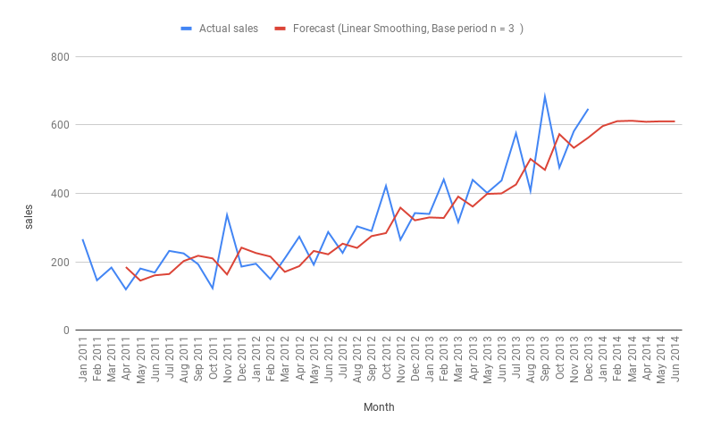
Performance Evaluation
- Calculated for 3 months period
- Percent of Accuracy Calculation (POA) = 87.20
- Mean Absolute Deviation (MAD) = 68.77
- Periods best fit (PBF) is Dec 2012 to Feb 2013
Exponential Smoothing- forecast method
This method is similar to Linear Smoothing. For a better understanding of Exponential Smoothing let’s take the following example data. The general formula for Exponential Smoothing forecast is
    F t+1 = Ft + α ( At - Ft )
        where α is smoothing constant  0 <= α <= 1,
    At - Actual sales of time t
    Ft - Forecast sales value of time t.
    F t+1 - Forecast sales for time t +1   i.e. next period.
    Rewrite the formula to simplifying the calculation.
    F t+1 = αAt + (1 - α)  Ft    in this example α =0.3
| Month | Sales ( At ) | Forecast ( Ft ) | calculation |
|---|---|---|---|
| Jan 2011 | 266 | 266 | because no previous data available |
| Feb 2011 | 145.9 | 266 | = ( 0.3 x 266 ) + (0.7 x 266) |
| Mar 2011 | 183.1 | 230 | = ( 0.3 x 145.9) + (0.7 x 266) |
| Apr 2011 | 216 | = ( 0.3 x 183.1) + (0.7 x 230) |
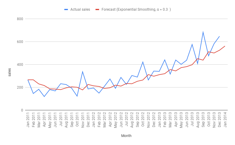
Performance Evaluation
- Calculated for 3 months period
- Percent of Accuracy Calculation (POA) = 87.20
- Mean Absolute Deviation (MAD) = 68.77
- Periods best fit (PBF) is Dec 2012 to Feb 2013
Conclusion
These illustrations may give you a good idea about forecasting strategies for improving the quality of prediction. part 1 of this article, covers 6 Simple Forecasting Methods. The incoming article we are going to discuss Exponential Smoothing with Trend and Seasonality, ARMA, ARIMA and more.
Find the calculation, preparation of these graphs of each sales forecasting methods. This may be useful for further references as a sales forecast template, using different forecasting methods with time series data Sales or demand forecast method demo with example data