Illustrating exponential smoothing time series forecasting - in examples

This article will illustrate exponential smoothing time series forecasting methods other than covered in part 1 and part 2. however, we are going to use the same dataset. Let’s get into the exponential smoothing models, with the explanation of formula, calculation, illustrated graph, and performance evaluation demonstration.

Types of exponential smoothing

There are three main types of exponential smoothing time series forecasting methods.

1. Single Exponential Smoothing / Simple Exponential Smoothing

Time series forecasting method depends only on previous observations of sales data without a trend or seasonality. It requires a single parameter, called alpha (a), Alpha (a) parameter - smoothing factor controls previous observations of sales or demand influence rate decay exponentially (value between 0 and 1.) * Max values (near to 1) - taking account to the most recent data * Min Value (near to 0) - more of the history is taken into account when making a prediction. This method was explained in our previous article

2. Double Exponential Smoothing

Exponential Smoothing that adds support for trends in the univariate time series. It requires beta (b) along with alpha (a) beta (b) parameter - smoothing factor controls the changes in trend influence rate to decay exponentially (value between 0 and 1.) * Additive Trend: Double Exponential Smoothing with a linear trend. * Multiplicative Trend: Double Exponential Smoothing with an exponential trend.

3. Triple Exponential Smoothing

Exponential Smoothing that adds support for seasonality to the univariate time series. This method is also called Holt-Winters Exponential Smoothing, to represent the contributors of this method Charles Holt and Peter Winters. It requires gamma (g) along with alpha (a) and beta (b) gamma (g) parameter - smoothing factor controls the influence on the seasonal component. * Additive Seasonality: Triple Exponential Smoothing with a linear seasonality. * Multiplicative Seasonality: Triple Exponential Smoothing with an exponential seasonality. We are going to see more details explanation about this method below.

Holt-Winters Exponential Smoothing

This method needs calculated values of the Seasonal index (S), the exponentially smoothed Average (A) or Level and the exponentially smoothed trend (T) from the sales order history.

How to calculate Seasonal index (S)

                      Sales of Jan 2013 + Sales of Jan 2012 
S (jan)  = --------------------------------------------------------------  x   12 
                      Total sales of 2013 +  Total sales of 2012    

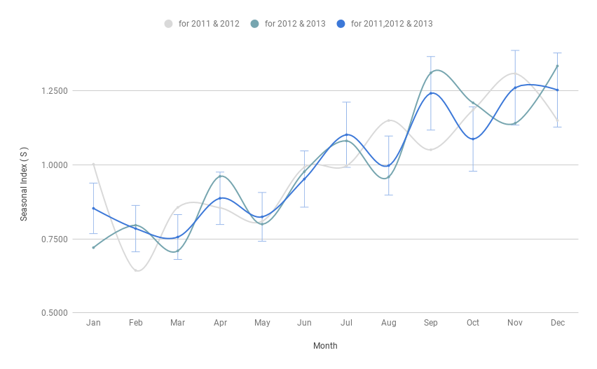
Below graph shows the calculated Seasonal index (S) from sales data of 2011, 2012 & 2013.

1. Seasonal index for 2011 & 12,
2. Seasonal index for 2012 & 13,
3. Seasonal index for 2011, 2012 & 2013,

How to calculate exponentially smoothed Average (A)

Smoothed Average At = α (Dt/St-L) + (1 - α)(At-1 + Tt-1)

                             Sales (Feb 2013) 
A (Feb 2013)  = α  ( --------------------------------- ) +  (1 - α)  ( A (Jan 2013)  + Trend  (Jan 2013) )
                             Seasonal index (Feb 2013)     

α smoothing coefficient   value range   0 < α < 1  

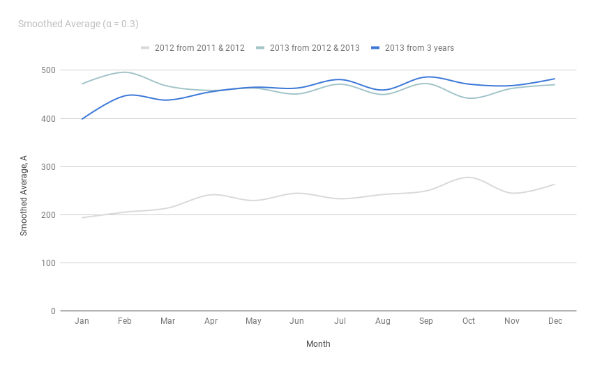
Below graph shows the calculated Smoothed Average (A) from sales data of 2011, 2012 & 2013. Here we used value for α = 0.3.

1. Smoothed Average for 2012
2. Smoothed Average for 2013 from values of 2012 & 2013 sales data.
3. Smoothed Average for 2013 from values of 2011, 2012 & 2013 sales data.

How to calculate exponentially smoothed Trend (T)

Smoothed Trend Tt = β (At - At-1) + (1 - β)Tt-1

T (Feb 2013)  = β ( Smoothed Average A (Feb 2013)  - s.a A (Jan 2013) ) + (1 - β) Trend(Jan 2013)

β smoothing coefficient   value range   0 < β < 1  

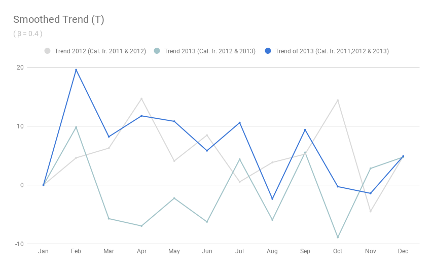
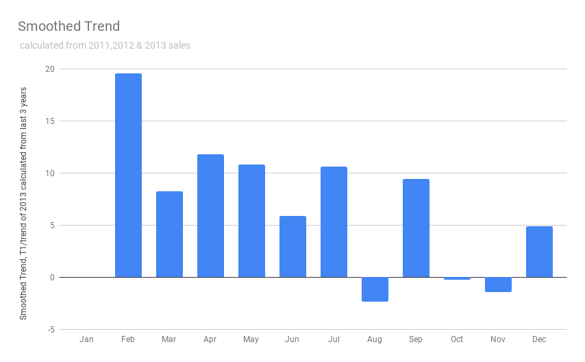
Below graph shows the calculated Smoothed Trend (T) from sales data of 2011, 2012 & 2013. Here we used value for β = 0.4

  1.  Smoothed Trend for 2012 
  2.  Smoothed Trend for 2013 from values of 2012 & 2013 sales data. 
  3.  Smoothed Trend for 2013  from values of 2011, 2012 & 2013 sales data.

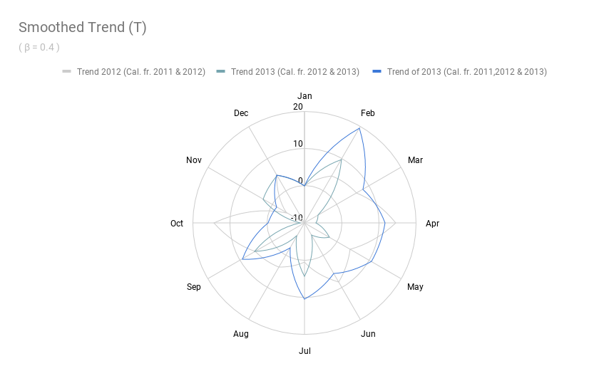
For better comparison, we used the graph radar chart. Generally, this data has a positive trend from Feb to Jul, Sep, and Dec. A negative trend in Aug, Oct, Nov.

How to forecast using smoothed Average, Trend, & Seasonal index

Forecast Ft+n = (At + (Tt) n)St-L+n

    At - Smoothed Average value of time t  
    Tt - Smoothed Trend value of time t. 
    F t+n - Forecast sales for time t +n   
    St - Seasonal index value of time t    
    n = Future period value 

F(Feb 2014)  =  ( Average A (Dec 2013) + ( Trend T(Dec 2013) ) x 2 ) x  Season Index (Feb 2013) 
  ,,
  ,,
F(Dec 2014)  =  ( Average A (Dec 2013) + ( Trend T(Dec 2013) ) x 12 ) x  Season Index (Dec 2013) 

Below graph shows the calculated Forecast (F)

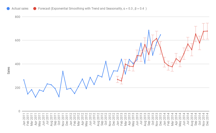
Performance Evaluation

• Calculated for 3 months period
• Percent of Accuracy Calculation (POA) = 96.37
• Mean Absolute Deviation (MAD) = 92.21
• Periods best fit (PBF) is Apr 2012 to Jun 2013

Conclusion

These exponential smoothing forecasting method illustrations may give you an idea about Seasonal index (S), the exponentially smoothed Average (A) or Level and the exponentially smoothed trend (T). Strategies to fine tune these factors to improving the quality of prediction.

Find the calculation, preparation of these graphs of each sales forecasting methods. This may be useful for further references as a sales forecast template, using different forecasting methods with time series data Sales or demand forecast method demo with example data